Editorial

Dr Prasanth V
Editor

 

Data and Variables

We often note the name, age and gender of our patients in case record forms. Most of the people are bothered about their body weight. All these attributes are called ‘variables’. A variable is simply what is being observed or measured. In other words attributes of patients and clinical events that vary and can be measured is called as a ‘variable’. As the name implies, variables vary among the members (units of observation) of a ‘population of interest’ and if they don’t vary, they become ‘constants’. In ‘165 centi-meters of height’, ‘height’ is the variableand ‘165 centimeters’ is the data. Statistics addresses variability.

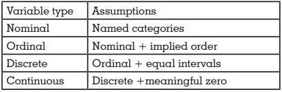
Variables are classified in many ways. Basically they are either ‘qualitative / categorical’ or ‘quantitative’ in nature . ‘Qualitative’ variables can be ‘nominal’, ‘binary/dichotomous’ or ‘ordinal’. Nominal variables are just named categories with no implied order among them. Gender, type of removable prosthesis delivered etcare examples of nominal variables because it doesn’t matter whether we say male or female first and it doesn’t matter whether we say Removable Partial Denture or Complete Denture first. ‘Binary or dichotomous’ variables are a type of ‘nominal variables’ where there are only two mutually opposite and exclusive options like ‘yes/no’ or ‘live/dead or ‘prosthesis present/absent’. ‘Ordinal’ variables on the other hand have an implied order unlike ‘nominal’ variables, but the difference between successive categories may not be equal. Stages of cancer and type of bone quality are classical examples. Cancer staging according to severity is expressed from Stage I to Stage IV, we can’t say stage IV before stage II. But the difference in severity between Stage 1 and II may not be same as the difference between stage II and IV. ‘Quantitative’ variables are measured in numerical values and they can be either ‘discrete’ or ‘continuous’. If data is available only in fixed intervals of whole numbers, variable is of ‘discrete’ type. Most of the scales like GCS, IQ, number of teeth present etc are examples of discrete variables. Even though the difference between successive categories are the same, true or meaningful ‘zero’ value may be absent here. Temperature in degree Celsius is a classic example. Zero degree Celsius doesn’t mean there is no temperature (it is the temperature at which water freezes) and hence 50 degree Celsius is not the half of 100 degree Celsius, but the difference between 25 and 50 degrees are same as the difference between 50 and 75 degrees. Hence we can say that only addition and subtraction are possible if variable is ‘discrete’. But if data can be obtained in continuum, variable is termed ‘continuous’. Examples include height, weight, fasting blood sugar, available bone etc. Here addition, subtraction, division and multiplication of data values are meaningful simply because there is a true and meaningful zero. 0 Kg weight means, there is no weight and 50 Kg is exactly the half of 100 Kg.

Continuous data is the most superior form of data followed by discrete, ordinal and nominal. We can always downgrade a data, but upgradation of data is normally not possible. Always try to collect the data in superior form. For example, when you are collecting the age of study participants, collect the exact age in years, months and days (as continuous) and never as completed age (as discrete)or age groups (as ordinal). This is because we can convert continuous data to discrete or ordinal if and when needed, but we can never do a reverse process. Nominal variables are measured in ‘nominal scale’, ordinal variables in ‘ordinal scale’, discrete variables in ‘interval scale’ and continuous variables in ‘ratio scale’. High ordinal variables (semi quantitative variables) like GCS categories can be analyzed in interval scale. As a general statement we can say that the nominal or ordinal data are restricted to ‘non-parametric’ statistics.

Variables can be ‘dependent’ or ‘independent’. Outcome of interest which changes in response to our intervention is called ‘dependent / outcome’ variable. The factor which s manipulated is called ‘independent/ exposure/predictor’ variable. ‘Dependent’ variables change in response to ‘independent’ variables. If we assess the crestal bone level six months following the osteotomy using conventional and bone expansion techniques, crestal bone level is the dependent variable and the two techniques compared become independent variables. But if we study the relationship between crestal bone level and implant failure, crestal bone level will become the ‘independent’ variable and implant failure, the ‘dependent’ variable. Now you may have understood very well that the same variable can become dependent or independent variable depending on the research question or on what you really study. If dependent variables are mediated through a third set of variables, the latter is called ‘intermediate variable’. For example, in case if crestal bone height is mediated through gingival inflammation, then gingival inflammation becomes the ‘intermediate’ variable. A more explanatory example will be the study on coronary heart disease resulting from increased salt intake which is mediated through hypertension.

Salt intake → hypertension → coronary heart disease
(Independent) (intermediate) (dependent)
Variables can be ‘composite’ or ‘baseline’. It is logical to understand and height and weight are ‘baseline’ variables and BMI which includes both height and weight is a ‘composite’ variable.‘Hard outcome’ variables like death, complete connector fracture etc do not result in any bias. ‘soft outcome’ variables like pain, peri implantitis etc are difficult to measure and hence can result in bias. Condition of liver can be directly assessed by a biopsy. But most often we resort to liver function tests to indirectly assess its status. Liver enzyme value, thus is a ‘proxy variable’.

Other variables, may be part of the system under study and may affect the relationship between independent and dependent variables are known as ‘extraneous variables (covariates)’. They are called so because they are extraneous to the research question, but may be part of the phenomenon under study. Few covariates can even be ‘confounders’ or ‘effect modifiers’. In depth discussion on those topics will be beyond the scope of this editorial.

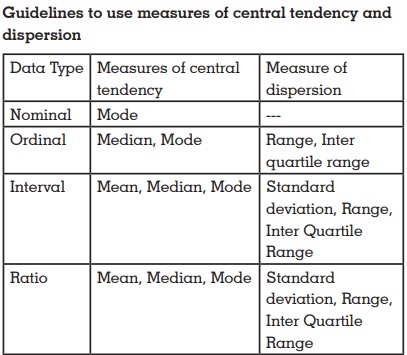
Why identification of variables is important?
Descriptive and inferential statistical methods used are different for different types of variables. Summary measures used, graphical representations used and types of statistical tests used are unique for each type of variable.



Bar diagrams and pie charts are useful for summarizing qualitative data. Histograms, frequency polygon, leaf and stem plot, box plot, scatter plot etcare useful for quantitative data. McNemar’s chi square test is useful for qualitative paired variables. Paired t and RM ANOVA are useful for quantitative paired variables withWilcoxon Signed Rank test and Friedman’s test being their non-parametric variants. Chi square test and correlation are used for unpaired qualitative and quantitative variables respectively. ANOVA and its two sample version, unpaired t test are useful for comparison of sample means. Less robust Z test which is based on stronger assumptions can substitute unpaired t test,only is sample size is large. Mann-Whitney U test and Kruskal Wallis H test are the non-parametric variants of unpaired t and ANOVA tests respectively.

Even though concept of variables and data are important in research,sometimes we may interpret few datainter changeably. For example, IQ, which is most likely an ordinal variable is interpreted as interval variable by most. Like Geoffrey R. Norman and David L. Streiner stated ‘as far as we know, they have not been arrested for doing so, nor has the sky fallen on their heads’.

Test your knowledge

Systolic BP – Continuous (though we collect as discrete values)
Age group – Ordinal (there is an order)
Completed age – Discrete (always a whole number)
Age – Continuous (need not be whole numbers)
Gender – Nominal (we can say any gender first)
BMI Categories – Ordinal (there is an order)
Rank in exam – Ordinal (Even though rank is given as 1,2,3….., it’s just a number to denote an order of merit. Rank 2 doesn’t mean that he/she has only half knowledge/mark than Rank 1)
RBC Count – Discrete (only whole numbers are possible)

References